Stroke Prediction Model
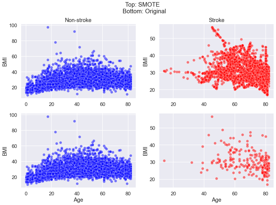
I tested 4 different models to see which model best predicts an instance of stroke in a patient based on several factors such as BMI and age. I used SMOTE (Synthetic Minority Over-sampling Technique) to change the unbalanced data to balanced data set by oversampling the minority class (stroke patient) data.
Goal
To predict stroke in patients based on their health and lifestyle data.
Data
The dataset is taken from Kaggle. It contains the following variables.
| Index | Column Name | Data Type | Description |
|---|---|---|---|
| 1. | 'gender' |
Categorical | Male/Female/Other |
| 2. | 'age' |
Numeric | Range of 0.08 (presumably babies) to 82 years old |
| 3. | 'hypertension |
Binary | 0/1 |
| 4. | 'heart_disease' |
Binary | 0/1 |
| 5. | 'ever_married' |
Binary | Yes/No |
| 6. | 'work_type' |
Categorical | ‘Private’, ‘Self-employed’, ‘Govt_job’, ‘children’, ‘Never_worked’ |
| 7. | 'Residence_type' |
Categorical | ‘Urban’, ‘Rural’ |
| 8. | 'avg_glucose_level' |
Numerical | 55.12- 274.74. Normal Adult range: 90-110 mg/dL |
| 9. | 'bmi' |
Numerical | 10.3 - 97.6. 18-25 is considered healthy |
| 10. | 'smoking_status' |
Categorical | ‘formerly smoked’, ‘never smoked’, ‘smokes’, ‘Unknown’ |
Results
Model 1: Simple logistic regression.
The logistic model that was trained on unbalanced data had a very high accuracy of 96%. However this is because accuracy measures the number of total correct predictions. Since the data had more non-stroke patients, it could accurately predict non-strokes, but that is not our goal. The high accuracy of model 1 only shows that the model is good at predicting non-stroke cases. Instead, we are far more interested in the number of stroke patients the model can predict.
from sklearn.metrics import confusion_matrix

cnf_matrix = confusion_matrix(y_train, lr_model.predict(x_train))

def plot_confusion_matrix(cm, classes,
                          normalize=False,
                          title='Confusion matrix',
                          cmap=plt.cm.Blues):
    """
    This function prints and plots the confusion matrix.
    Normalization can be applied by setting `normalize=True`.
    """
    import itertools
    if normalize:
        cm = cm.astype('float') / cm.sum(axis=1)[:, np.newaxis]
        print("Normalized confusion matrix")
    else:
        print('Confusion matrix, without normalization')

    print(cm)

    plt.imshow(cm, interpolation='nearest', cmap=cmap)
    plt.title(title)
    plt.colorbar()
    tick_marks = np.arange(len(classes))
    plt.xticks(tick_marks, classes, rotation=45)
    plt.yticks(tick_marks, classes)

    fmt = '.2f' if normalize else 'd'
    thresh = cm.max() / 2.
    for i, j in itertools.product(range(cm.shape[0]), range(cm.shape[1])):
        plt.text(j, i, format(cm[i, j], fmt),
                 horizontalalignment="center",
                 color="white" if cm[i, j] > thresh else "black")

    plt.tight_layout()
    plt.ylabel('True label')
    plt.xlabel('Predicted label')

class_names = ['No Stroke', 'Stroke']
# Plot non-normalized confusion matrix
plt.figure()
plt.grid(False)
plot_confusion_matrix(cnf_matrix, classes=class_names,
                      title='Confusion matrix')

# Plot normalized confusion matrix
plt.figure()
plt.grid(False)
plot_confusion_matrix(cnf_matrix, classes=class_names, normalize=True,
                      title='Normalized confusion matrix')
Even though Model 1 showed a high accuracy of 0.96 when predicting the y_train data, the model faired very poorly on predicting true positives.
Model 2: Simple logistic regression on SMOTE transformed data.
Model 2 was trained on the SMOTE transformed data which reduced accuracy to 95% from model 1. Although accuracy was reduced, the number of true positives increased from 0 to 22.
Model 2 uses the same logistic regression model as Model 1, except the data used has been transformed using SMOTE. Here is the code I used for oversampling data on stroke patients.
sm = SMOTE(random_state=42)

X_sm, Y_sm = sm.fit_resample(X, Y)

print(f'''Shape of X before SMOTE: {X.shape}
Shape of X after SMOTE: {X_sm.shape}''')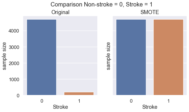
We can see that SMOTE successfully increases the size of data on stroke patients.
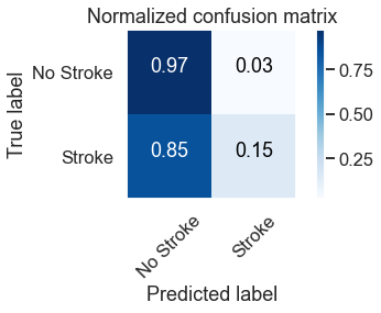
We see here that we have slightly increased our stroke predictions to 15% , up from 0%. Model 2 also misdiagnosed 3% of patients (93 / 5110 rows) to have stroke when they actually did not have stroke.
Model 3: Logistic regression (with feature engineering).
Model 3 was trained on the SMOTE transformed data and cut from 22 features to only 5 features. This was done through the process of feature engineering where the results of the first n-features were iteratively tested to
-
maximise true positives
-
minimise false positives
-
minimise cross entropy loss
It was found that the logistic regression model that have the first 5 features had the best performance.
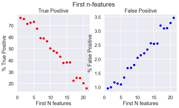
The 5 feature SMOTE logistic regression model is the best performing logistic regression model so far. It predicted 73% of the actual stroke cases (True Positives) and gave a false stroke diagnosis to 27% of the stroke cases (False Positives).
Model 4: K-nearest neighbour classification.
I have found that the K-nearest neighbour classification for k=4,5,6 gave the highest true positive score of 100% (predicted 100% of actual stroke cases) and the lowest false positive score of 4% (wrongly classified healthy paitents as at risk of stroke).
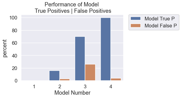
Summary
Models used:
| Model | Model Description | True Positive (%) & Number | False Positive (%) & Number |
|---|---|---|---|
| 1 | Logistic Regression trained on original data | 0% (0) | 0% (0) |
| 2 | Logistic Regression trained on SMOTE data | 16% (10) | 3% (31) | 3 | Logistic Regression trained on first 5 features | 70% (44) | 26% (298) |
| 4 | K-nearest neighbour classification | 100% (63) | 4% (44) |
In the absence of a perfect model that correctly identifies stroke and non-stroke cases, the next best model should prioritise a high percentage of stroke diagnosis, even if this means wrongly diagnosing someone who does not have stroke. This is because it would be more devastating to tell someone they are not at risk of a stroke when they actually do, than to tell a healthy patient they are at risk of stroke when they are not. In other words, it would be better to err on the side of caution.