Mathematical Modelling & Urban Planning: Lowry’s Pittsburgh Model
When I was in university, I read a paper that used math for urban planning. I remember choosing to take that urban studies class because it was non-technical, so I was quite surprised to see math equations in one of my readings. When I was looking for something to write about for my first blog post, I decided it would be on that paper - “A Model of Metropolis” by Ira S. Lowry.
In it, Lowry proposed a computational model to help urban planners optimally allocate land for housing and retail businesses. He figured computers would be helpful for a big task like planning a city, given all the variables one needs to consider like transportation, housing and workplaces. This was the 1960s, so using computers was still a pretty novel idea. His model took in the current locations of all workplaces in Pittsburgh and would output the optimal land-use for both housing and retail businesses across the city of Pittsburgh. Some sources call it a ‘demand-driven model’ because the model allocated housing based on demand from workers who wanted to live near to their workplaces. The model also allocated retail businesses based on the potential demand from housing areas. In other words, the logic was: workers drive the demand for housing which in turn drive the demand for retail businesses like supermarkets. The location of housing and retail businesses also had to satisfy quality of life requirements like minimising commute times and not exceed some housing density threshold.
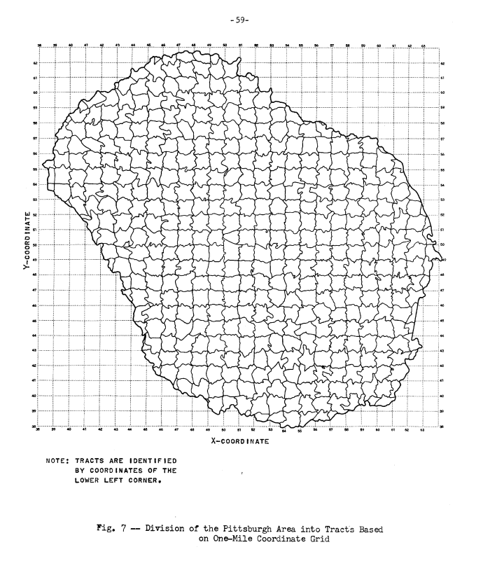
At beginning of modelling process, Lowry divided Pittsburgh into 1-sq mile pieces that he called ‘tracts’.
The area within the $j$-th tract was a sum of areas for 4 land-use types, represented by equation (1).
\[\large \begin{align} A_j &= A_j^U + A_j^B + A_j^R +A_j^H \tag{1}\\ \end{align}\]Where,
-
$U$: Usable but unoccupied land
-
$B$: Basic sector (business)
-
$R$: Retail sector (business)
-
$H$: Household sector (residential)
Lowry defined each land-use type as such:
-
Basic sector. This land-use type is made up of businesses that primarily serve clients outside the city. This category is designed to be unaffected by the movement of the local population, in contrast to the retail sector.
-
Retail sector. This land-use type consists of businesses in the city that generate revenue from the local population. This implies that the more people live in or near a tract, the more retail sector businesses there ought to be. For instance, fewer households in the tract would mean fewer schools (Lowry counts public services as ‘retail’) and supermarkets nearby.
-
Household sector. The number of households in the area, which the retail sector is dependent on.
-
Unoccupied Land. Self-explanatory.
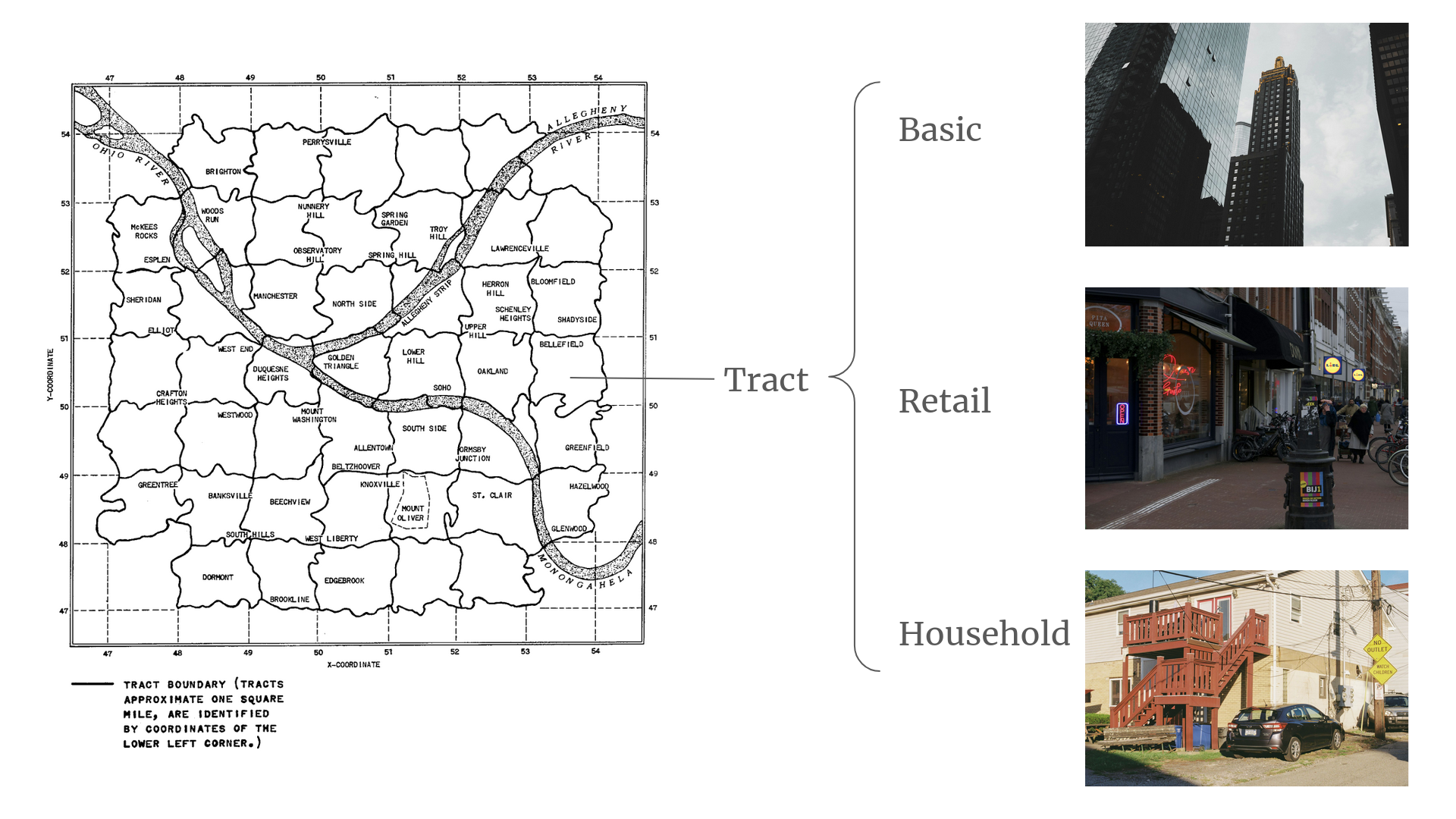
(Left: An image from the paper with the tract divisions. Right: The three categories plus unoccupied land which is not shown.)
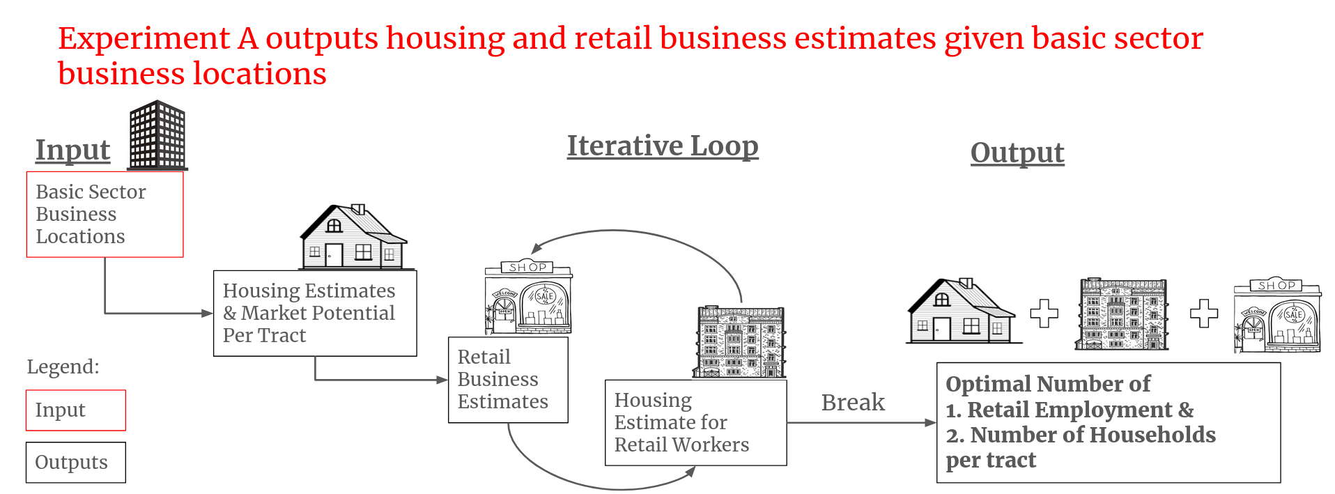
The algorithm starts with the input of basic sector businesses locations. The algorithm then undergoes a “part-waterfall-part-iterative” process which outputs two sets of data. One, the number of households and two, the number of retail businesses which should be in each tract. I’ll describe what the “waterfall” and “iterative” processes are.
At the waterfall step, the model distributes housing across the city based on the location of basic sector businesses. In the algorithm, the housing locations are distributed in such a way that houses are close enough to workplaces but without exceeding some housing density threshold to prevent overcrowding. Given that most basic sector businesses are located in the city centre, housing is distributed out of the city centre radially to satisfy the housing density threshold. Equations 8 and 11 of the model represent the objective and constraint respectively.
Equation 8 minimises commute time.
\[\large \begin{align} N_j &= g \sum^n_{i=1} \frac{E_i}{T_{ij}} \tag{8} \\ \end{align}\]Where,
-
$N_j$ is the housing population in the tract $j$
-
$g$ is some unspecified coefficient,
-
$E_j$ is the number of employment opportunities in tract $i$
-
$T_{ij}$ is the pairwise distance between tracts $i$ and $j$.
Equation (8) tells us the population in each tract will increase if there are more employment opportunities within a short distance. Lowry is assuming people will buy houses near their workplaces. A large $N_j$ implies many jobs (large $E_i$) within a short distance (small $T_{ij}$) of tract $j$.
Equation 11 suppresses housing density to prevent overcrowding in the tracts.
\[\large \begin{align} \frac{N_j}{A^H_j} &\leq Z^H_j\tag{11} \\ \end{align}\]Where,
-
$N_j$ is the housing population in the tract $j$
-
$A^H_j$ is the area of land-use assigned to housing
-
$Z^H_j$ is the arbitrary population density cap to avoid overcrowding.
Here, Lowry sets an arbitrary population density ratio $Z_j^H$. The ratio between population to area in tract $j$ cannot exceed this ratio.
(Remarks: I rewrote the original equation (11) for ease of reading. The full set of equations and the table of notations are found below.)
After the area allocated for housing in each tract is determined, the “market potential” of each tract is calculated. Lowry defined “market potential” as the initial estimate of how many retail businesses are required to supply goods and services to households in that tract and surrounding tracts.1 Lowry added in the ‘surrouding tracts’ bit to factor in the possibility that people living at the edge of their own tract boundary may choose to visit neighbouring tracts to buy things. Up till here, the algorithm can be viewed as a waterfall process. After this, it enters the iterative step.
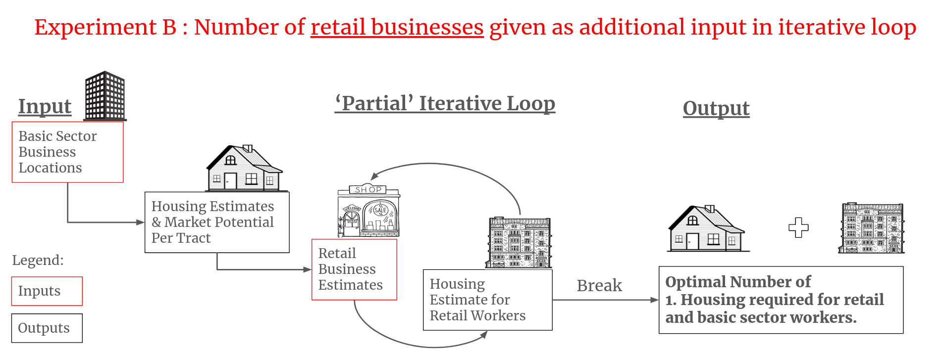
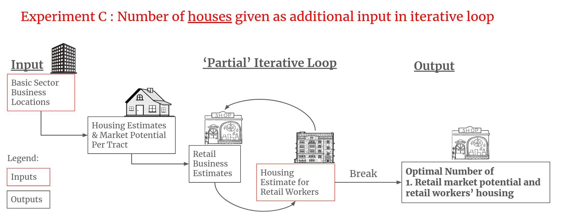
At the iterative step, the model enters a loop to assign the number of retail businesses based on the calculated market potential and subsequently assigns housing for retail workers. The loop breaks when all retail workers are housed and all constraints are satisfied. Explained briefly, the constraints ensure that each retail business serves a minimum number of customers to remain profitable, population density does not exceed a preset number and all areas sum up to the total area of available land. A fuller explanation of the iterative step constraints are listed in equations (10) - (11) of the full model below.
I’ve broken the model roughly into four groups, area ($A$), employment ($E$) and housing ($N$) and constraints. However, there are some interaction equations that cannot be neatly classified in any one group.
Notations
| Decision Variable Notations | Meaning |
|---|---|
| $A$ | Area of land (thousand square feet) |
| $E$ | Employment (number of persons) |
| $N$ | Population (number of households) |
| $T$ | Index of trip distribution |
| $Z$ | Constraints |
| Super/Subscript Notations | Meaning |
|---|---|
| $U$ | Usable Land |
| $B$ | Basic Sector |
| $R$ | Retail Sector |
| $H$ | Household Sector |
| $k$ | Retail sector/Shopping trip class. Examples of a class include ‘Food and Drugs’, ‘Department Stores’ etc. |
| $m$ | number of classes of retail establishments ($k = 1, …,m$); Lowry used m=10. |
| $i, j$ | Sub-areas of a bounded region, called tracts |
| $n$ | Number of tracts ($i=1,…,n; j =1,…n$) |
Unspecified functions and coefficients: $a,b,c,d,e,f,g$
Full Model
Area
\[\large \begin{align} A_j &= A_j^U + A_j^B + A_j^R +A_j^H \\ \tag{1} \end{align}\](1) The area within the $j$-th tract is a sum of areas for 4 land-use types: Usable but unoccupied land, basic sector, retail sector, housing.
Employment
\[\large \begin{align} E^k &= a^k N \tag{2} \\ E^k &= b^k \left[\sum^n_{k=1} \left(\frac{c^kN_i}{T_{ij}^k} + d^k E_j\right)\right] \tag{3}\\ E^k &= \sum^n_{j=1} E^k_j \tag{4} \\ E_j &= E_j^B + \sum^m_{k=1} E^k_j \tag{5} \\ A^R_j &= \sum^m_{k=1} e^k E_j^k \tag{6} \end{align}\](2) $E^k$ denotes the employment for the $k$-th retail sector, a function of how many people live in the area. Lowry supposed that the more people lived in the area, the more employment required in the retail sector. $a^k$ is a weight that represents the market potential of the given location.
(3) The RHS expresses employment as a measure of distance between homes and shopping areas. $\left(\frac{c^kN_i}{T^k_{ij}}\right)$ is a ratio of the number of residents in tract $i$ to a score of the distance between tracts $i$ and $j$. It is a confusing but reasonable assumption that people will travel to neighbouring tracts for shopping if it’s not very far away.
(4) The total employment in the $k$-th retail sector is the sum of employment in the $k$-th retail sector in all tracts
(5) Sum of all retail sectors employment and basic sector employment is the total employment for each tract.
(6) Land required for retail is a function of employment figures. More employees = more business = more land for retail needed.
Housing
\[\large \begin{align} N &= f \sum^n_{j=1} E_j \tag{7}\\ N_j &= g \sum^n_{i=1} \frac{E_i}{T_{ij}} \tag{8} \\ N &= \sum^n_{j=1} N_j \tag{9}\\ \end{align}\](7) The region’s population of households is a function of employment. The assumption here is that people can only live if they have jobs to pay for housing.
(8) The number of households in a tract is a function of distance to employment opportunities. The \(T_{ij}\) term handles the pair-wise distance between tracts.
(9) Sum of residents in all tracts must equal total population count.
Constraints
\[\large \begin{align} E_j^k &\geq Z^k \hspace{0.5cm} \text{, or else $E_j^k=0$} \tag{10} \\ N_j &\leq Z^H_jA^H_j \tag{11} \\ A^R_j &\leq A_j - A^U_j -A^B_j \tag{12} \end{align}\](10) Retail employment must hit a minimum number otherwise it will be set to zero. This simulates a minimum economies of scale for retail businesses to be profitable.
(11) The population density of a tract is suppressed by this equation. The greater the accessibility of the tract, the lower the population density.
(12) Amount of land used for retail cannot exceed available land (which equals the sum of land in the $j$ -th tract minus all other land use areas)
Results
Lowry used a 1958 census dataset as input for his model and also a source of comparison. The dataset contained the actual number of houses, retail and basic sector businesses in each tract. He could not use the dataset to validate his model since his model recommended how the city should be planned, so differences would obviously be expected. The most he could do was compare the differences and speculate about the causes of discrepancy if there were any. Still, I think it’s interesting to read of how Lowry designed three experiments to compare the 1958 dataset and his model’s output. I’ve summarised each of the experiments below.
| Experiment | Input | Output |
|---|---|---|
| A | - Basic employment figures - Land use data |
Distribution of retail employment and household figures |
| B | - Basic and Retail figures |
Distribution of household figures |
| C | - Retail employment figures - Land use data |
Retail employment & market potential |
Experiment A was the full model run: Basic sector business locations were given as inputs and the model would output how much household and retail businesses there should be per tract. Experiment B and C were partial runs to test the iterative logic of the model. In Experiments B and C, Lowry and his team inserted either ground-truth numbers of housing or retail business at the iterative step instead of allowing the model to propose its own solution. This was done to speed up convergence and to see if there was any difference between partially ‘aided’ solution and ‘unaided’ solution.
Although there was no causal evidence, Lowry claimed that his model predicted a rise in population in the western area of Pittsburgh. Lowry wrote that his model did not consider road networks in the city and so housing was allocated symmetrically between the Eastern and Western areas of the city. Whereas, in the 1958 dataset, more people were living in the Eastern areas because the Western area lacked road infrastructure. However, in the years between 1958 and his paper, Lowry observed that The Fort Pitt Tunnel and a road linking to the Greater Pittsburgh Airport led to rapid growth in population and employment in the western area of Pittsburgh.2 I am not convinced that this is evidence for the usefulness of Lowry’s model as a predictive tool. I would think a better comparison would have been to compare between the model’s outputs before and after the Fort Pitt Tunnel and extra roads were added. But, I don’t think they had sufficient computational power to add in road networks to their model.
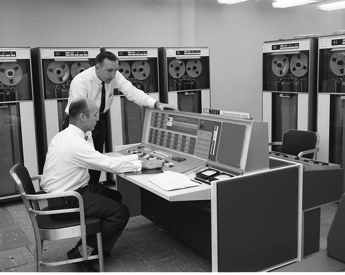
A photo of an IBM 7090, the computer model used to run Lowry's simulations.
Overall, I am skeptical about possibility to predict the future impact of city planning decisions given the large number of variables that affect where people choose to live, work and shop. I might be wrong because when I googled “Lowry Pittsburgh Model”, there were many other land-use models which were derivatives of Lowry’s Pittsburgh Model. Some were even implemented in other countries. You can read more about them here, assuming you’re still interested in land-use planning models at this point.
I think the paradox of using computational models for urban planning can be stated as something like, “Planning a city takes a lot of time and money. Therefore, we should model the effects well enough so that we don’t realise a big mistake after we’ve finished building.” The flipside is, “Planning a city takes a lot of time, so we are not sure how much of the model’s predictions will be outdated by the time we’ve finished building” For example, pro-work-from-home policies might shift people away from living in the city center where rent is higher. People are also increasingly moving to online shopping which reduces the demand for physical retail businesses in the area. All these are possible reasons for model drift. Add to that the difficulty of consolidating different types of data to update the model and you have a difficult problem for folks in urban planning, operations research, sociology, mathematics, economics and even a bored liberal arts graduate to write about.
Thanks to Dominic Ko, Matthew Ling, Andrew Siow, Nicole Lai and Michelle Ong for reading drafts of this. Shoutout to A/P Chaewon Ahn for introducing me to urban data science.
Footnotes
-
Market potential is the linear combination of the number of workplaces and the number of households in that tract and adjoining tract. The coefficients depend on how far the tract is, this applies for adjacent tracts. For workplaces, coefficients are infinite for distances greater than one mile. ↩
-
The Fort Pit Tunnel was opened in 1960, two years after the 1958 dataset was compiled. It was featured in the book and film, “The Perks of Being a Wallflower.” ↩
